DPO: RLHF collapsed into one loss
In May 2023, a paper showed up titled “Direct Preference Optimization: Your Language Model is Secretly a Reward Model.” (Rafailov et al. 2023) The claim: you could do RLHF without a reward model, without PPO, without rollouts, and without RL training of any kind. Just preference pairs and a clever loss function.
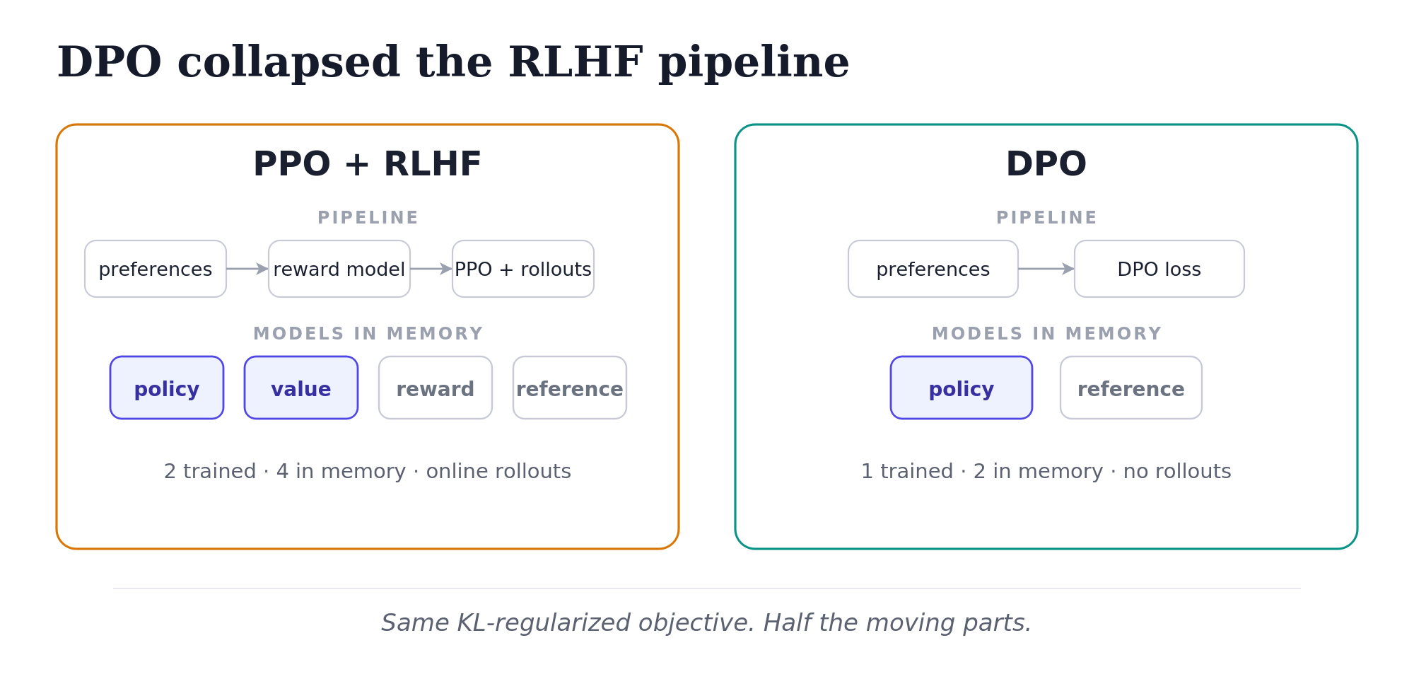
If you’d been working with PPO + RLHF up to that point, this sounded too good to be true. PPO was famously painful. Four models in memory simultaneously: policy, value network, reference model, reward model. Online sampling during training. The Anthropic and OpenAI teams running serious RLHF had built infrastructure most people couldn’t afford to replicate.
DPO said: skip all of it. Train a single supervised loss on preference pairs. Done.
I followed DPO when it landed. I derived the math step by step. I wrote a small training pipeline around TRL’s DPOTrainer and got it running locally on a 24GB GPU. In parallel, the community’s reaction was also immediate: within months, the open-source preference-tuning ecosystem had largely shifted to DPO. Models like Zephyr (Tunstall et al. 2023) showed up. The teams running PPO infrastructure didn’t go away, but the floor opened up dramatically.
In this article, let me first anchor what DPO is replacing.
Why PPO + RLHF was painful
PPO + RLHF is a multi-stage pipeline. You start with an SFT model, then:
- Collect a preference dataset: pairs of (prompt, chosen response, rejected response).
- Train a separate reward model on this dataset, learning to score (prompt, response) pairs.
- Run PPO using the reward model as the reward signal, generating fresh rollouts during training.
Training requires four LLM-sized models in memory: the SFT model serves as the reference for KL anchoring, the policy is the LLM model being trained, the reward model scores rollouts, and PPO needs a value network on top.
The KL anchor matters because of what happens without it. The policy will drift toward outputs that score high under the reward model but bear no relationship to coherent text. Reward models, being LLMs themselves, have adversarial inputs: sequences that exploit weaknesses in the reward model and produce arbitrarily high scores while reading as gibberish. The KL term keeps the policy close to the SFT model.
Mathematically, the RLHF objective is:
\[\max_\pi \; \mathbb{E}_{x \sim D, \, y \sim \pi(\cdot|x)} \left[ r(x, y) - \beta \log \frac{\pi(y|x)}{\pi_\text{ref}(y|x)} \right]\]
In words: maximize expected reward, subject to a KL penalty that keeps you close to the reference model. The hyperparameter \(\beta\) controls the tradeoff.
This objective has a closed-form optimal policy, and that closed form contains all the information you need to train against preference data directly: no reward model, no rollouts, no PPO. We’ll work through the derivation in a few paragraphs. But first, the conceptual move.
The DPO surprise
DPO’s pitch is structural. The RLHF pipeline has two coupled training problems: train a reward model that captures human preferences, then use that reward model to train a policy. DPO observes that these two steps are mathematically linked. Specifically, given the KL-regularized RLHF objective above, the optimal policy can be expressed as a function of the reward.
If you can express the reward in terms of the optimal policy, you don’t need to train a reward model separately. You can plug the implicit reward directly into the preference modeling framework, and now your policy is being trained to match preferences directly.
The result: a single supervised loss on preference pairs. No rollouts. No value network. No reward model.
Two models in memory: the policy being trained, and the reference model. That’s it. Compare to PPO + RLHF’s four. The memory and simplicity savings are significant.
But before showing the math, I want to land the right intuition for what DPO is doing.
The key intuition: relative to the reference
The wrong reading of DPO: “It’s preference training. Increase chosen, decrease rejected.” Roughly what happens, but it misses the structural point.
DPO doesn’t push chosen up and rejected down in absolute terms. If the reference already strongly preferred chosen, DPO barely moves; if it was indifferent or wrong, DPO pushes hard.
This is what preserves the KL anchor from RLHF. Naive preference training (just push chosen up, rejected down) would let the policy drift arbitrarily far from the reference. The “above what the reference already was” part is what keeps DPO solving the same KL-regularized problem PPO + RLHF solves. And it’s free: the KL anchor falls out of the derivation. No separate KL term in the loss.
The derivation: where the DPO loss comes from
I’m going to walk through this in four steps.
Step 1: Start from the KL-regularized RLHF objective
Same objective as PPO + RLHF:
\[\max_\pi \; \mathbb{E}_{x \sim D, \, y \sim \pi(\cdot|x)} \left[ r(x, y) - \beta \log \frac{\pi(y|x)}{\pi_\text{ref}(y|x)} \right]\]
We want high reward, but we pay a penalty for drifting too far from the reference model. The hyperparameter \(\beta\) trades off these two pressures.
Step 2: Solve for the optimal policy
The KL-regularized objective above has a closed-form solution. After working through the calculus (the partition function manipulation is the heart of it), the optimal policy is:
\[\pi^*(y|x) = \frac{1}{Z(x)} \pi_\text{ref}(y|x) \exp\!\left(\frac{1}{\beta} r(x, y)\right)\]
where \(Z(x) = \sum_y \pi_\text{ref}(y|x) \exp\!\left(\frac{1}{\beta} r(x, y)\right)\) is a normalizer that makes the result a valid probability distribution.
The optimal policy is the reference policy tilted toward high-reward completions, with the strength of the tilt controlled by \(\beta\).
This step is doing real algebraic work. Deriving it requires writing the objective as a KL divergence between two distributions and identifying the minimizer. For a more granular walk-through of the derivation, see my earlier write-up at https://chanys.github.io/dpo/. For the conceptual flow, what matters is the form: the optimal policy is the reference, multiplied by an exponentiated reward term, normalized.
Step 3: Rearrange to express reward through the policy
The expression in Step 2 has reward on the right and optimal policy on the left. We can flip it. Take the log of both sides:
\[\log \pi^*(y|x) = \log \pi_\text{ref}(y|x) + \frac{1}{\beta} r(x, y) - \log Z(x)\]
Solving for \(r(x, y)\):
\[r(x, y) = \beta \log \frac{\pi^*(y|x)}{\pi_\text{ref}(y|x)} + \beta \log Z(x)\]
This is the “your language model is secretly a reward model” moment. The reward function, the thing we were going to train a separate reward model to estimate, can be expressed entirely in terms of the optimal policy and the reference policy. No reward model needed. The reward is encoded in the log-probability ratio between the optimal policy and the reference policy.
The partition function \(Z(x)\) is still hanging around, which is annoying because computing it requires summing over all possible completions \(y\). We’ll deal with it in the next step.
Step 4: Plug into Bradley-Terry
The Bradley-Terry preference model gives the probability that one response is preferred over another, in terms of their rewards:
\[p(y_w \succ y_l \mid x) = \sigma\big(r(x, y_w) - r(x, y_l)\big)\]
where \(\sigma\) is the logistic sigmoid. Substituting in our expression for \(r(x, y)\) from Step 3:
\[p(y_w \succ y_l \mid x) = \sigma\!\left( \beta \log \frac{\pi^*(y_w|x)}{\pi_\text{ref}(y_w|x)} - \beta \log \frac{\pi^*(y_l|x)}{\pi_\text{ref}(y_l|x)} \right)\]
The partition function disappeared. Bradley-Terry only cares about reward differences between two completions for the same prompt, and \(Z(x)\) depends only on the prompt: it cancels out in the subtraction. This is the reason DPO works as a practical algorithm. Without this cancellation, we’d be stuck computing partition functions over the full output space.
We replace \(\pi^*\) with our learned policy \(\pi_\theta\) and minimize the negative log-likelihood of the observed preferences:
\[L_\text{DPO}(\theta) = -\,\mathbb{E}_{(x, y_w, y_l) \sim D} \left[ \log \sigma\!\left( \beta \log \frac{\pi_\theta(y_w|x)}{\pi_\text{ref}(y_w|x)} - \beta \log \frac{\pi_\theta(y_l|x)}{\pi_\text{ref}(y_l|x)} \right) \right]\]
This is the DPO loss. Run gradient descent on it over a preference dataset, and you’re solving the same KL-regularized RLHF objective that PPO was solving; without the reward model, the rollouts, or the value network.
What the loss is actually doing
Look at the structure of the DPO loss. There are two log-probability ratios: one for the chosen response, one for the rejected. Each compares the current policy’s probability to the reference policy’s probability. The loss wants the chosen log-ratio to be larger than the rejected log-ratio.
This is the formal version of the intuition I described earlier. The training pressure is to increase the chosen-over-rejected log-ratio relative to the reference, not to increase chosen and decrease rejected in absolute terms. If the reference model already gave higher probability to the chosen response, the loss is already partially satisfied; the gradient is small. If the reference was wrong (gave higher probability to the rejected response), the gradient is large, pushing hard against the reference.
The KL anchor is built into the structure of the loss, not a separate term. Both numerators in the log-ratios are the policy being trained; both denominators are the reference. The reference’s behavior is the implicit constraint on what the policy can do.
The original RLHF objective had a KL penalty as an added term. DPO collapses everything: the reward, the KL anchor, the policy update; into a single supervised loss where the structure of the equation enforces all three.
What DPO meant for the field
Rather than replacing online RL, DPO carved out a specific lane. What DPO won is the open-source ecosystem of budget-constrained preference tuning: for teams without lab-scale compute, DPO is the dominant approach. The structural distinction that matters is online (fresh rollouts during training) vs. offline (a fixed preference dataset), not PPO vs. DPO. Online has an exploration advantage; offline is simpler. For most use cases, the simplicity wins.
In mid-2023, doing RLHF was something a small number of well-resourced labs could do. PPO was complex and engineering-intensive. The infrastructure for online preference tuning was confined to teams that had built it. Most people who wanted to fine-tune a model on preference data couldn’t realistically do it.
By late 2023, that had changed. DPO + qLoRA + 4-bit quantization meant the entire preference-tuning recipe could be run on a single GPU. The Zephyr models, the Tülu series, the wave of open instruction-tuned models that followed: all of these were downstream of DPO making the pipeline accessible. The simplification of preference tuning meant orders of magnitude more people could do it.
Appendix: Deriving the optimal policy
This is the gory derivation I deferred in Step 2: the manipulation that takes the KL-regularized RLHF objective and produces the closed-form optimal policy. I worked through this in late 2023, a few months after the DPO paper came out, because I wanted to convince myself the algorithm was real rather than take the result on faith. What follows is essentially that derivation, cleaned up. Skip this section if you’re satisfied with the form of the result. Read on if you want to see how the partition function shows up.
We start with the RLHF objective:
\[\max_\pi \; \mathbb{E}_{x \sim D, \, y \sim \pi(\cdot|x)} \left[ r(x, y) - \beta \log \frac{\pi(y|x)}{\pi_\text{ref}(y|x)} \right]\]
The KL divergence can be written as an expectation:
\[\mathbb{D}_\text{KL}\!\left[\pi(y|x) \,\|\, \pi_\text{ref}(y|x)\right] = \mathbb{E}_{y \sim \pi(\cdot|x)}\!\left[ \log \frac{\pi(y|x)}{\pi_\text{ref}(y|x)} \right]\]
So the inner expectation in our objective becomes:
\[\mathbb{E}_{y \sim \pi(\cdot|x)}\!\left[ r(x, y) - \beta \log \frac{\pi(y|x)}{\pi_\text{ref}(y|x)} \right]\]
Divide by \(-\beta\) to convert the maximization into a minimization, and the sign of the reward term flips:
\[\min_\pi \; \mathbb{E}_{x \sim D} \, \mathbb{E}_{y \sim \pi(\cdot|x)}\!\left[ \log \frac{\pi(y|x)}{\pi_\text{ref}(y|x)} - \frac{1}{\beta} r(x, y) \right]\]
Use the identity \(x = \log \exp(x)\) to rewrite the reward term:
\[\min_\pi \; \mathbb{E}_{x \sim D} \, \mathbb{E}_{y \sim \pi(\cdot|x)}\!\left[ \log \frac{\pi(y|x)}{\pi_\text{ref}(y|x)} - \log \exp\!\left(\frac{1}{\beta} r(x, y)\right) \right]\]
Combine the two logarithms:
\[\min_\pi \; \mathbb{E}_{x \sim D} \, \mathbb{E}_{y \sim \pi(\cdot|x)}\!\left[ \log \frac{\pi(y|x)}{\pi_\text{ref}(y|x) \exp\!\left(\frac{1}{\beta} r(x, y)\right)} \right]\]
The denominator inside the log isn’t a probability distribution: it doesn’t sum to one over \(y\). We can fix this by introducing a normalizer \(Z(x)\):
\[Z(x) = \sum_y \pi_\text{ref}(y|x) \exp\!\left(\frac{1}{\beta} r(x, y)\right)\]
and defining:
\[\pi^*(y|x) = \frac{1}{Z(x)} \pi_\text{ref}(y|x) \exp\!\left(\frac{1}{\beta} r(x, y)\right)\]
By construction, \(\pi^*\) is a valid probability distribution: it’s nonnegative everywhere and sums to one over \(y\). Now we substitute it back into our objective. Add and subtract \(\log Z(x)\) inside the bracket (no change, since these cancel):
\[\min_\pi \; \mathbb{E}_{x \sim D} \, \mathbb{E}_{y \sim \pi(\cdot|x)}\!\left[ \log \frac{\pi(y|x)}{\pi_\text{ref}(y|x) \exp\!\left(\frac{1}{\beta} r(x, y)\right)} + \log Z(x) - \log Z(x) \right]\]
Use the identity \(\log Z(x) = -\log \frac{1}{Z(x)}\) on the first \(\log Z(x)\) term:
\[\min_\pi \; \mathbb{E}_{x \sim D} \, \mathbb{E}_{y \sim \pi(\cdot|x)}\!\left[ \log \frac{\pi(y|x)}{\pi_\text{ref}(y|x) \exp\!\left(\frac{1}{\beta} r(x, y)\right)} - \log \frac{1}{Z(x)} - \log Z(x) \right]\]
Combine the first two log terms using \(\log a - \log b = \log(a/b)\):
\[\min_\pi \; \mathbb{E}_{x \sim D} \, \mathbb{E}_{y \sim \pi(\cdot|x)}\!\left[ \log \frac{\pi(y|x)}{\frac{1}{Z(x)}\, \pi_\text{ref}(y|x) \exp\!\left(\frac{1}{\beta} r(x, y)\right)} - \log Z(x) \right]\]
Recognize the denominator inside the log as \(\pi^*(y|x)\):
\[\min_\pi \; \mathbb{E}_{x \sim D} \, \mathbb{E}_{y \sim \pi(\cdot|x)}\!\left[ \log \frac{\pi(y|x)}{\pi^*(y|x)} - \log Z(x) \right]\]
The \(\log Z(x)\) term doesn’t depend on \(\pi\), so it’s a constant with respect to the optimization. We can drop it. What’s left is exactly a KL divergence:
\[\min_\pi \; \mathbb{E}_{x \sim D}\!\left[ \mathbb{D}_\text{KL}\!\left[\pi(y|x) \,\|\, \pi^*(y|x)\right] \right]\]
KL divergence is minimized when the two distributions are equal. So the minimizer is \(\pi = \pi^*\):
\[\pi^*(y|x) = \frac{1}{Z(x)} \pi_\text{ref}(y|x) \exp\!\left(\frac{1}{\beta} r(x, y)\right)\]
That’s the closed-form optimal policy. The rest of the DPO derivation (Steps 3 and 4 in the main text) follows from rearranging this expression to extract the implicit reward and plugging it into Bradley-Terry.
The partition function \(Z(x)\) is the technical price of admission for this derivation. It would be intractable to compute directly as it requires summing over all possible completions, but it cancels out in the final DPO loss because Bradley-Terry only cares about reward differences. That cancellation is what makes DPO work as a practical algorithm.