GRPO: the algorithm behind reasoning models
In January 2025, DeepSeek released R1 (Guo et al. 2025): a reasoning model that closed most of the gap to OpenAI’s o1 at a fraction of the training cost, and (more importantly) shipped with the training recipe described in the open. The recipe centered on an algorithm called GRPO. Within a few months, essentially every open-source reasoning model (Qwen’s reasoning variants, Llama derivatives, the wave that followed) was using GRPO or close cousins of it.
GRPO itself wasn’t new in 2025. The DeepSeek team had introduced it a year earlier, in their DeepSeekMath paper (Shao et al. 2024), where they used it to train a 7B math-specialist model. What changed in 2025 was the demonstration that the same algorithm could produce general reasoning capability at frontier scale.
If you’ve been trying to understand how reasoning models like o1, R1, or their successors actually get trained, GRPO is most of the answer. This post is about what GRPO is, why it works, and where it sits relative to the PPO + RLHF recipe it (sometimes) replaces.
I’m assuming you already understand PPO at the level of the previous post in this series. That assumption matters because GRPO is best understood as a small, deliberate set of changes from PPO, not as a new algorithm built from scratch. Most of what makes PPO work (clipping, importance sampling, the multi-epoch inner loop) carries over unchanged. The changes are concentrated in two places.
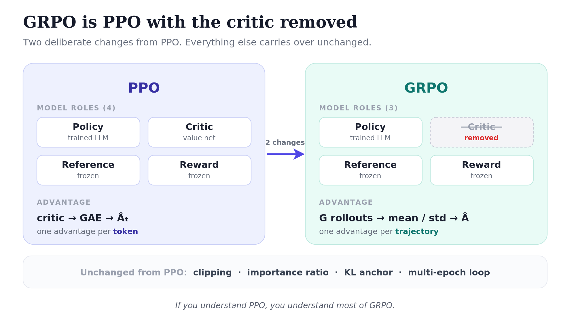
Here’s the short version of GRPO: GRPO is PPO with the critic removed. Instead of using a value network to estimate per-token advantages, GRPO samples multiple rollouts per prompt and computes each rollout’s advantage relative to its siblings.
That’s the whole conceptual move. One model gone from memory. Per-token advantage replaced with per-trajectory advantage. Everything else stays. Which raises the question of why this works at all, and why it works especially well for reasoning.
Why drop the critic?
In PPO, four model roles are active during training:
- Policy: the LLM being trained
- Value network: the critic, also trained, typically same architecture as the policy
- Reference model: frozen copy of the SFT model, for KL anchoring
- Reward model: frozen, scores complete responses
That’s four LLM-sized things in the picture. The actual memory cost depends on a lot of implementation details (whether the policy and value share a body, how parameters are sharded across GPUs, optimizer state for the trained models) but the structural fact stands: PPO involves four model roles, and reducing that count is a real win.
Two of those roles you can’t avoid. The reference model is structurally necessary; without it you have no KL anchor and the policy drifts into reward-hacking gibberish. The reward model (or verifier) provides the training signal in the first place.
But the value network? It’s only there to compute advantages. If you can compute advantages another way, you can drop it.
A natural question is whether the reward model could just take over. It can’t.
The reward model and the value network do fundamentally different jobs. The reward model answers: “How good is this complete response?” It takes a (prompt, response) pair and outputs a scalar. It was trained on human preferences over finished outputs, so it has no signal for half-finished responses. The value network answers a different question: “Given this partial state, what total reward do I expect by the end?” It takes a state (prompt plus tokens-so-far) and predicts where things are heading.
These are different questions. One scores finished things. The other predicts where things are heading. The reward model can’t do the second job because no human ever rated half-responses during preference data collection.
So the value network isn’t redundant. PPO needs it because GAE (the per-token advantage estimator) needs to know the expected outcome at every state along the trajectory, and only the value network can provide that.
Rather than substitute the reward model for the value network, GRPO gives up on per-token advantage estimation entirely.
Group-relative advantages
Here’s the new advantage computation. For each prompt, generate \(G\) rollouts (typically 4 to 16). Score each one with the verifier. The advantage of the \(i\)-th rollout is:
\[\hat{A}_i = \frac{r_i - \text{mean}(r_1, \ldots, r_G)}{\text{std}(r_1, \ldots, r_G) + \epsilon}\]
That’s it. Each rollout gets one scalar advantage (“how much better than my sibling rollouts did this one do?”) applied identically to every token in that rollout.
This is a different kind of advantage than what PPO uses. PPO had a different advantage per token, derived from GAE; GRPO has the same advantage for every token in a rollout, derived from how the rollout’s reward compared to its siblings’. The credit is assigned at the trajectory level, not the token level. That’s the cost of dropping the value network: less granular credit assignment. But it’s also why GRPO works without per-token value estimates.
Let me make this concrete with the example I’ll use throughout: training a model to solve grade-school math word problems.
“Maya is buying tickets for a concert. Adult tickets cost $12 each and child tickets cost $8 each. She buys 9 tickets total and spends $92. How many adult tickets did she buy?”
The answer is 5. The verifier extracts the model’s final boxed answer and checks: 1 if correct, 0 if not.
Sample 4 rollouts (\(G = 4\)):
- Rollout A: sets up the equation \(12a + 8(9-a) = 92\), solves cleanly, ends with
\boxed{5}. Reward: 1. - Rollout B: tries \(a + c = 9\) and \(12a + 8c = 92\) but makes an arithmetic slip, ends with
\boxed{6}. Reward: 0. - Rollout C: solves it correctly via testing values, ends with
\boxed{5}. Reward: 1. - Rollout D: confuses adult and child prices, ends with
\boxed{4}. Reward: 0.
Compute the group statistics. The mean is straightforward:
\[\text{mean} = \frac{1 + 0 + 1 + 0}{4} = 0.5\]
For the standard deviation, take squared deviations from the mean and sum them:
\[(1 - 0.5)^2 + (0 - 0.5)^2 + (1 - 0.5)^2 + (0 - 0.5)^2 = 4 \times 0.25 = 1.0\]
Then divide by \(G - 1 = 3\) (only 3 of the 4 deviations are independent once the mean is fixed) and take the square root:
\[\sigma = \sqrt{1.0 / 3} \approx 0.577\]
(Some implementations divide by \(G\) instead, giving \(\sigma = 0.5\). The choice rescales all advantages by the same factor and doesn’t change their signs, but it can matter when comparing hyperparameters across codebases.)
Advantages are then \((r_i - \text{mean}) / \sigma\):
- \(\hat{A}_1 = (1 - 0.5) / 0.577 \approx +0.866\) (rollout A)
- \(\hat{A}_2 = (0 - 0.5) / 0.577 \approx -0.866\) (rollout B)
- \(\hat{A}_3 = (1 - 0.5) / 0.577 \approx +0.866\) (rollout C)
- \(\hat{A}_4 = (0 - 0.5) / 0.577 \approx -0.866\) (rollout D)
In the gradient update, every token in rollouts A and C gets multiplied by \(+0.866\), and every token in rollouts B and D gets multiplied by \(-0.866\). The policy gets pushed toward the trajectories that solved the problem, away from the ones that didn’t.
The intuition is clean: of these attempts, which ones got it right? Reinforce those.
What happens when all rollouts score the same
A subtle but important case. If all 4 rollouts get reward 0 (model failed every attempt), or all 4 get reward 1 (model succeeded every time), then the standard deviation is 0, the mean equals every \(r_i\), and every advantage is 0.
This is the algorithm correctly saying “there’s no learning signal here.” If all attempts failed, we don’t know which failures were closer to success. If all succeeded, we don’t know which successes were genuinely well-reasoned versus lucky. Either way, no rollout in this group is “better than its siblings,” so no gradient signal gets generated.
The practical implication: GRPO is most effective when the model is at a difficulty level where it sometimes succeeds and sometimes fails. Too easy and all rewards are 1; too hard and all rewards are 0. Either way, no signal. Training data needs to sit in the model’s “frontier” of difficulty, which is why curriculum learning matters more for GRPO than it does for PPO.
Everything else looks PPO-shaped
With the advantage computed, the rest of the algorithm is structurally identical to PPO.
The clipped policy loss has the same form as PPO. Same importance ratio:
\[r_t(\theta) = \frac{\pi_\theta(a_t \mid s_t)}{\pi_{\theta_\text{old}}(a_t \mid s_t)}\]
Same min-of-clipped-and-unclipped construction for the per-token policy loss:
\[\ell^\pi_t = -\min\!\Big(r_t(\theta) \cdot \hat{A}_t,\; \text{clip}(r_t(\theta), 1-\epsilon, 1+\epsilon) \cdot \hat{A}_t\Big)\]
The only difference from PPO: \(\hat{A}_t\) is now the trajectory-level group-relative advantage rather than the token-level GAE advantage. Every token in a given rollout shares the same \(\hat{A}_t\). Clipping mechanism, importance ratio, asymmetric min; all unchanged.
The multi-epoch inner loop is the same: collect rollouts, do \(K\) epochs of mini-batched gradient steps, discard, repeat.
KL anchoring is also the same idea, though implemented differently. PPO often folds the KL term into the per-token rewards before computing advantages. GRPO can’t easily do this, as rewards in GRPO arrive only at the end of each rollout, with no per-token reward to fold into. So GRPO adds the KL as a separate per-token loss term:
\[\ell^{\text{KL}}_t = \log \pi_\theta(a_t \mid s_t) - \log \pi_\text{ref}(a_t \mid s_t)\]
This is the simple log-ratio estimator of KL; same as PPO uses. The two per-token losses then combine into a single scalar that gets backpropped:
\[L_\mathcal{B} = \frac{1}{|\mathcal{B}|} \sum_t \Big[\ell^\pi_t + \beta \cdot \ell^{\text{KL}}_t\Big]\]
Two separate per-token loss components, summed with a weight \(\beta\), averaged across all tokens in the mini-batch. Both contribute their own gradients to the policy parameters.
If you understand PPO, you understand most of GRPO. Two things change: how the advantage gets computed, and what models are in memory. Everything else carries over.
Why this works for reasoning specifically
GRPO didn’t have to be a reasoning algorithm. The math is generic. You could use it for any task with a scalar reward at the end. But there’s a structural reason it works especially well for reasoning.
Reasoning tasks have two properties that are awkward for PPO:
Rewards are usually verifiable. Math problems have right answers. Code can be tested. The reward is a deterministic check (“did the code pass the tests?”), not a learned approximation of human preferences. This is the world of Reinforcement Learning with Verifiable Rewards (RLVR) and it’s the world GRPO was made for.
Reward is genuinely sparse. You don’t know if a chain of thought is good until you see whether it produced the right final answer. Intermediate tokens can look identical between a trajectory that ends correctly and one that ends wrong, until the very end.
PPO handles sparse rewards via the value network, which has to learn “how good does this partial reasoning trajectory look?” That’s a hard regression problem. Reasoning trajectories can look identical for many tokens, then diverge wildly at the answer. The value network struggles to fit this signal cleanly, and the resulting advantages are noisy.
GRPO sidesteps the problem entirely. It compares whole rollouts to each other rather than trying to predict per-token value.
There’s also a practical reason GRPO and verifiable rewards pair well. GRPO needs \(G\) rollouts per prompt to compute group statistics: meaning the reward function gets called \(G\) times per prompt. If the reward function is a few lines of Python that runs in microseconds (a math correctness checker, a code test runner), scaling to \(G = 16\) is free. If the reward function is a 7B-parameter reward model requiring a full forward pass, \(G\times\) inference cost gets expensive fast. GRPO’s economics work in the verifier setting.
This is also where the practical scope of “verifiable” matters. Verifiable rewards work cleanly for math (correctness check on the final answer), code (test cases), formal proofs (proof assistants), and constrained generation (regex compliance). They don’t work for tasks like “is this response helpful?” or “is this writing tasteful?”. Those are inherently subjective and need RLHF-style learned rewards. So GRPO + RLVR complements RLHF for a specific (and increasingly important) class of tasks rather than replacing it for general assistant training.
What R1-Zero showed
When DeepSeek published the R1 paper in early 2025, they actually published two models, and the distinction is informative.
DeepSeek-R1 is the deployable model. Trained with a multi-stage pipeline: cold-start SFT, then GRPO + RLVR, then more SFT, then more RL. This is the one people actually use.
DeepSeek-R1-Zero is the surprising one. Trained with pure RL (GRPO + verifiable rewards) directly on the DeepSeek-V3 base model, with no SFT stage at all. R1-Zero showed that reasoning behavior could emerge from RL alone, without any supervised demonstrations of how to reason. The DeepSeek paper documents the specific behaviors that emerged during training:
- Generating progressively longer chains of thought as training continued: the model learning, as training progresses, that more inference-time compute helped it solve harder problems.
- Reflecting on its own solutions, revisiting and evaluating earlier reasoning steps.
- Exploring alternative approaches when a first attempt didn’t pan out.
- Critiquing intermediate steps and catching its own errors.
None of this was programmed in. The RL process simply rewarded the model for producing correct answers in the right format, and the rest emerged. The DeepSeek paper calls this a “self-evolution”: the model learning, through exploration and reward, how to reason without ever being shown an example.
R1-Zero’s outputs were rough at the surface. The model would mix languages mid-response (sometimes Chinese in the middle of an English answer), use inconsistent formatting, occasionally produce incoherent passages. That’s what made the deployable R1 require additional SFT stages on top, to clean up the surface presentation while keeping the reasoning capability.
The R1-Zero result changed how people thought about what RL could do. The conventional wisdom had been that you needed SFT to give the model a starting distribution before any RL could help. R1-Zero showed that’s not strictly true for capabilities that have verifiable signals. Pure RL on a base model can produce reasoning. You don’t need to demonstrate how to reason, only to verify when it worked.
The current consensus pipeline for production reasoning models combines: SFT for assistant behavior, preference tuning for helpfulness/harmlessness/honesty, RLVR for reasoning capability. Each stage does a job the others can’t do well. R1-Zero showed the RL stage could work without the prior stages; R1 showed why production models include them anyway.
Where GRPO fits in the broader landscape
The post-training landscape as of 2026 has split into a few distinct lanes.
Frontier general RLHF (proprietary, OpenAI / Anthropic / Google) still uses PPO-based or proprietary variants of PPO. Frontier labs have the engineering resources to handle PPO’s complexity and care about every fraction of a percent of quality. PPO is online, it generates new rollouts and learns from them, whereas DPO is offline, learning from a fixed preference dataset. That exploratory advantage seems to matter at the frontier. The frontier labs don’t share their pipelines publicly, so it’s hard to know exactly what they do, but PPO and its descendants remain in use.
Open-source preference tuning has largely migrated to DPO and its variants. DPO is much simpler than PPO: no rollouts, no value network, no reward model, just a clever loss on preference pairs. For most open-source teams, the simplicity is worth more than whatever quality edge PPO might provide.
Reasoning models use GRPO + RLVR. This is the lane DeepSeek pioneered with R1, and most open-source reasoning models follow the same recipe.
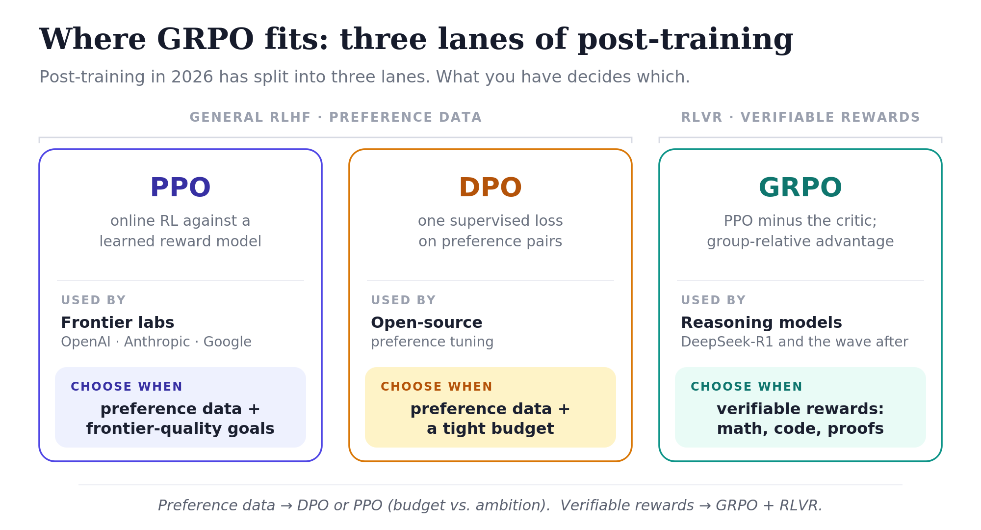
The practical takeaway: PPO and DPO/variants share the general-RLHF space (frontier vs open-source split); GRPO + RLVR owns reasoning. For practitioners, the choice depends on what you have. Preference data and a tight budget? DPO. Preference data and frontier-quality ambitions? PPO + RLHF. Verifiable rewards (math, code, theorem proving)? GRPO + RLVR.
Summary
In the broader arc that this post sits in, the next piece is DPO, the offline alternative that displaced PPO in much of the open-source ecosystem. Conceptually different from GRPO, DPO collapses the whole RL pipeline into a single supervised loss, but solves a related problem.
There’s a broader point worth naming here. PPO is hard. The four-models setup, the value network’s instability, and the sensitivity to hyperparameters are real engineering challenges. For years, these kept serious RL research mostly confined to a handful of well-resourced labs. GRPO did more than simplify an algorithm; it made RL training accessible to teams that couldn’t have run a stable PPO pipeline if they tried.