Eval scores are samples, not truth

How to tell real eval gains from noise.

Part of a series

LLM evaluation, honestly

1. Stop vibe-checking your agent
2. Read traces before you write the labeling guide
3. Don’t ask an LLM judge what code can check
4. Your LLM judge is a classifier
5. Eval scores are samples, not truth
6. Your RAG score hides the diagnosis
7. Your eval system also drifts

An eval score is a measurement from a sample, and samples are noisy. The dashboard reported 73% on Monday. By Friday it reported 75%. The team called it progress. But the eval set had 120 examples. The difference may just be noise.

Three habits cover most of the eval-noise problem:

1. Compare versions on the same examples.
2. Report uncertainty on the difference, not just the score.
3. Check whether the result is large enough to act on.

1. Compare versions on the same examples

When comparing two versions of a system, run them on the same eval set. If the samples differ, the result mixes two things: whether v8 is better, and whether v8 happened to get easier examples.

Suppose both versions are run on 300 traces:

• v7 passes 213 traces: 71%
• v8 passes 228 traces: 76%

The headline improvement is 5 percentage points. Before treating that as real progress, we need to ask how much uncertainty surrounds that estimate.

2. Report the CI of the difference

Because both versions ran on the same 300 traces, each trace falls into one of four outcomes:

Outcome	Count
Both pass	198
Both fail	57
v8 fixes a v7 failure	30
v8 breaks a v7 pass	15

The signal is in the disagreement rows. v8 fixes 30 cases and breaks 15, so the net gain is:

\[ \frac{30 - 15}{300} = 0.05 = 5\text{ percentage points} \]

Figure 1: The signal is in the disagreements. Running v7 and v8 on the same 300 traces, 255 are agreements (198 both pass, 57 both fail); these cancel and carry no signal (d = 0). Only the 45 disagreements move the number: 30 cases v8 fixed (d = +1) and 15 it broke (d = −1), a net of +15 traces, which is the observed +5 points.

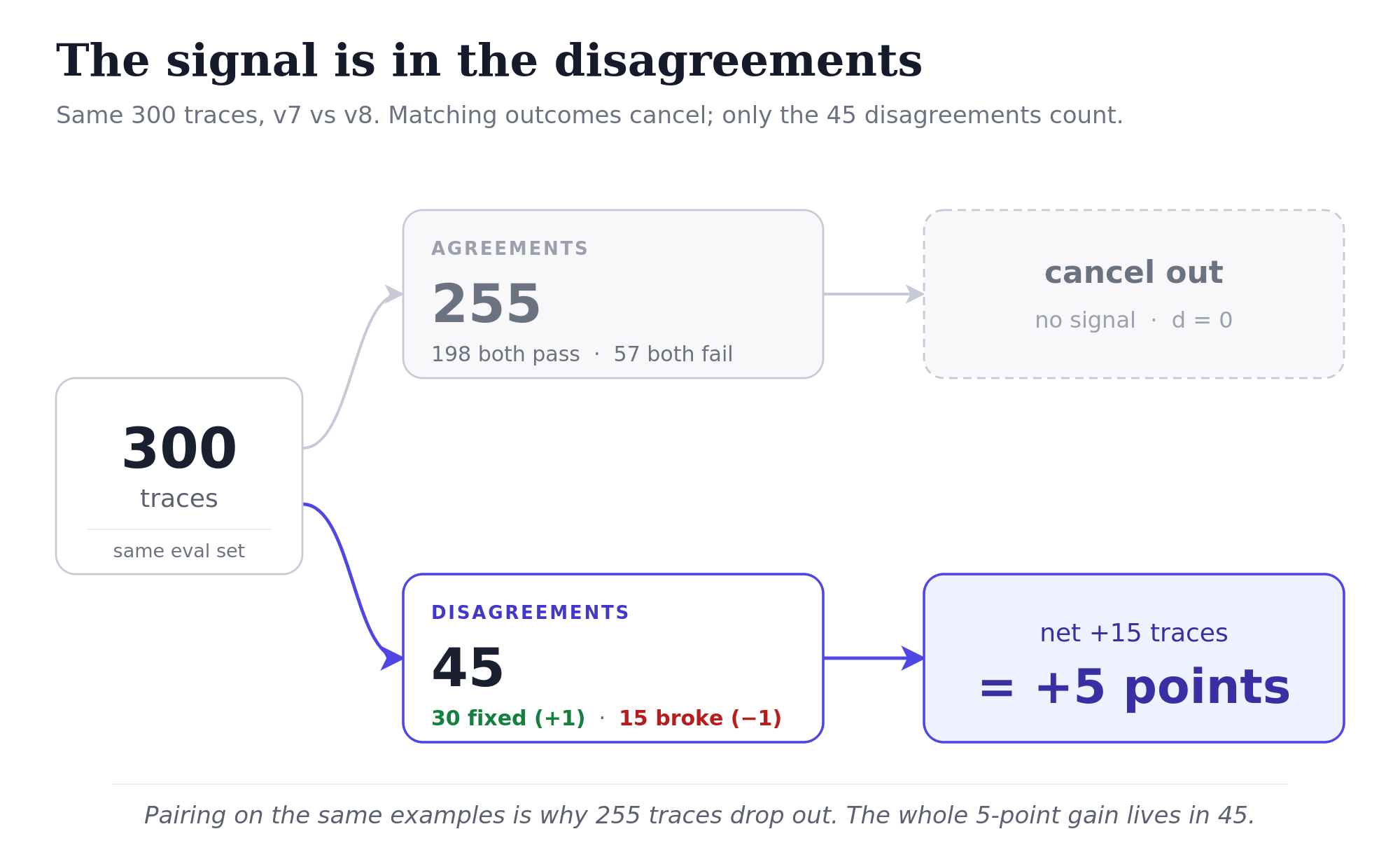
But this 5-point gain is still an estimate from one eval sample. If we drew another 300 traces, the measured improvement might be 3.8 points, 6.1 points, or 4.4 points. The confidence interval tells us how noisy the estimate is.

Step 1: Define the trace-level change

For each trace, define a before-and-after value \(d\):

\[ d = \begin{cases} +1 & \text{if v8 fixes a v7 failure} \\ -1 & \text{if v8 breaks a v7 pass} \\ 0 & \text{if both versions agree} \end{cases} \]

In this example:

\[ P(d=+1)=\frac{30}{300}=0.10,\quad P(d=-1)=\frac{15}{300}=0.05,\quad P(d=0)=\frac{255}{300}=0.85 \]

The expected value of \(d\), meaning the average trace-level change, is:

\[ \begin{aligned} E[d] &= P(d=1)(1) + P(d=-1)(-1) + P(d=0)(0) \\ &= (0.10)(1) + (0.05)(-1) + (0.85)(0) \\ &= 0.05 \end{aligned} \]

That matches the observed 5-point improvement.

Step 2: Compute the standard deviation

Standard deviation measures how spread out the trace-level changes are around their average.

To get it, first compute the variance:

\[ \mathrm{Var}(d) = E[d^2] - E[d]^2 \]

Compute \(E[d^2]\):

\[ \begin{aligned} E[d^2] &= \sum_x P(d=x) \cdot x^2 \\ &= P(d=+1)(+1)^2 + P(d=-1)(-1)^2 + P(d=0)(0)^2 \\ &= (0.10)(1)^2 + (0.05)(-1)^2 + (0.85)(0)^2 \\ &= 0.15 \end{aligned} \]

Then:

\[ \begin{aligned} \mathrm{Var}(d) &= E[d^2] - E[d]^2 \\ &= 0.15 - (0.05)^2 \\ &= 0.1475 \end{aligned} \]

Standard deviation is the square root of variance:

\[ \mathrm{SD} = \sqrt{0.1475} \approx 0.384 \]

So the individual trace-level changes have standard deviation about \(0.384\).

Step 3: Convert standard deviation into standard error

The standard deviation tells us how much individual trace outcomes vary. The standard error tells us how much the average improvement would vary across repeated eval samples.

A useful way to remember it:

\[ \mathrm{SE} = \frac{\mathrm{SD}}{\sqrt{N}} \]

Here:

\[ \begin{aligned} \mathrm{SE} &= \frac{0.384}{\sqrt{300}} \\ &\approx 0.022 \end{aligned} \]

So the standard error is 2.2 percentage points.

Step 4: Build the 95% confidence interval

For a rough 95% confidence interval, use the estimate \(\pm 1.96\) standard errors:

\[ \begin{aligned} \mathrm{CI} &= \text{improvement} \pm 1.96 \times \mathrm{SE} \\ &= 5.0\% \pm 1.96 \times 2.2\% \\ &= 5.0\% \pm 4.3\% \\ &\approx [0.7\%, 9.3\%] \end{aligned} \]

The interval excludes zero, but only barely. v8 is probably better than v7, but the estimate is not precise. The best estimate is a 5-point gain; the plausible range is roughly a 1-point to 9-point gain.

Compare the difference, not overlapping CIs

Do not decide whether v8 is better by checking whether the two individual confidence intervals overlap. For example:

• v7 pass rate: 71%, 95% CI [65.9%, 76.1%]
• v8 pass rate: 76%, 95% CI [71.2%, 80.8%]

These intervals overlap, but that is not the right test.

The right test is the confidence interval of the paired difference:

• v8 - v7 = +5 percentage points
• 95% CI of the difference = [0.7%, 9.3%]

This interval excludes zero, so the paired comparison says v8 is likely better.

Figure 2: Overlap is the wrong test. Top (the wrong test): v7’s pass-rate CI [65.9%, 76.1%] and v8’s [71.2%, 80.8%] visibly overlap, which naively reads as inconclusive. Bottom (the right test): the paired-difference CI, v8 minus v7 = +5 points with 95% CI [0.7%, 9.3%], sits entirely to the right of zero, so the paired comparison says v8 is likely better. Same data, opposite conclusions depending on the method.

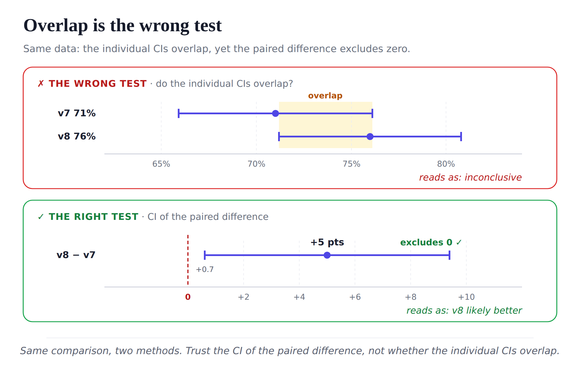
The paired comparison uses the trace-by-trace difference. Both versions were tested on the same examples, so the comparison removes a lot of noise from easy versus hard traces.

So when comparing two versions, report the CI of the paired difference. Do not rely on whether the individual pass-rate CIs overlap.

3. Know what this eval set can reliably detect

The confidence interval \(\mathrm{CI}\) tells us how uncertain this observed 5-point improvement is. The same standard error \(\mathrm{SE}\) also gives a rough planning number: how large an improvement this eval set can reliably detect.

A common rule of thumb is:

\[ \text{detectable improvement} \approx 2.8 \times \mathrm{SE} \]

The factor \(2.8\) comes from two requirements:

• First, the observed improvement has to be large enough that the 95% confidence interval excludes zero. With a normal approximation, that means the improvement is about \(1.96 \times \mathrm{SE}\) away from zero.
• Second, we do not want an eval set that detects the improvement only when we get lucky with the sample. We want enough power. Power means: if the improvement is real, how often would this eval setup detect it?

An eval with 80% power means that if the true improvement is exactly the size we care about, then repeated evals of the same size would detect it about 80% of the time.

To get 80% power, the true effect needs some extra margin beyond the 95% significance cutoff. Under the normal approximation, that extra margin is about \(0.84 \times \mathrm{SE}\).

So the rough detectable improvement is:

\[ \begin{aligned} \text{detectable improvement} &\approx (1.96 + 0.84) \times \mathrm{SE} \\ &\approx 2.8 \times \mathrm{SE} \end{aligned} \]

In plain English: the improvement should be large enough not merely to look significant in one lucky eval run, but to be detected reliably across repeated eval samples.

In the example above:

\[ \begin{aligned} \text{detectable improvement} &\approx 2.8 \times 2.2\% \\ &\approx 6.2\% \end{aligned} \]

So this 300-trace eval can reliably detect improvements around 6 percentage points under this disagreement pattern. The observed improvement is 5 points. v8 is probably better, but the evidence is borderline.

For paired pass/fail evals with a disagreement pattern similar to this example, the rough detectable improvement is:

• 100 traces: about 10 percentage points
• 300 traces: about 6 percentage points
• 1000 traces: about 3 percentage points

Figure 3: Small eval sets can’t see small gains. The smallest improvement an eval set can reliably detect is roughly 2.8 × SE (1.96 for significance plus 0.84 for power). Since SE = SD/√N, the detectable threshold is proportional to 1/√N: about 10 points at 100 traces, 6 at 300, 3 at 1000, and you need 4× the traces to halve it. Anything below the curve is the noise floor; the observed +5-point gain at 300 traces sits just inside it, which is why the evidence is borderline.

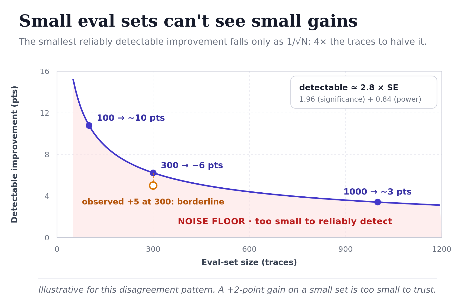
The exact numbers change with the disagreement rate, but the lesson is stable: small eval sets cannot reliably detect tiny improvements.

If v8 improves by 2 points on a small eval set, the honest conclusion is usually not “v8 is better.” It is “directionally positive, but too small to trust on this eval set.”

The same paired logic works for scored ratings

Not every eval is pass/fail. Sometimes humans score each output on a small scale, such as 1, 2, or 3.

The same paired logic still applies. For each example, compute the score difference:

\[ d_i = \text{score}_{v8,i} - \text{score}_{v7,i} \]

Now the possible values are wider:

\[ d_i \in \{-2, -1, 0, +1, +2\} \]

For example:

• \(1 \rightarrow 3\) gives \(d = +2\)
• \(2 \rightarrow 3\) gives \(d = +1\)
• \(2 \rightarrow 2\) gives \(d = 0\)
• \(3 \rightarrow 2\) gives \(d = -1\)

Then compute the average difference and its confidence interval the same way:

\[ \mathrm{SE} = \frac{\mathrm{SD}(d)}{\sqrt{N}} \]

\[ 95\%\,\mathrm{CI} = \bar d \pm 1.96 \times \mathrm{SE} \]

So if v7 averages 2.1 and v8 averages 2.6 on the same 300 examples, the mean paired improvement is \(+0.5\) points on the 1–3 scale. The confidence interval depends on how much the per-example differences vary.

What comes next

Three habits cover most of the eval-noise problem. Compare versions on the same eval set. Report the CI of the paired difference. Know your eval set’s noise floor before debating small movements.

The next article Your RAG score hides the diagnosis takes this to RAG evaluation: did retrieval find the right passage, did generation stay faithful to it, did the answer address what the user actually asked, did the system recognize when to decline. Collapsing those into a single “RAG quality” score loses these distinctions.

The next time someone celebrates a 2-point improvement, first ask: what is the CI, and how big is your eval set?